Chapter 2
The Power and Peril of Pictures
Visualizations
While we have been able to make several interesting observations about data by simply running our eyes down the numbers in a table, our task would have been much harder had the tables been larger. In data science, a picture can be worth a thousand numbers.
We saw an example of this earlier in the text, when we examined John Snow's map of cholera deaths in London in 1854.

Snow showed each death as a black mark at the location where the death occurred. In doing so, he plotted three variables — the number of deaths, as well as two coordinates for each location — in a single graph without any ornaments or flourishes. The simplicity of his presentation focuses the viewer's attention on his main point, which was that the deaths were centered around the Broad Street pump.
In 1869, a French civil engineer named Charles Joseph Minard created what is still considered one of the greatest graph of all time. It shows the decimation of Napoleon's army during its retreat from Moscow. In 1812, Napoleon had set out to conquer Russia, with over 400,000 men in his army. They did reach Moscow, but were plagued by losses along the way; the Russian army kept retreating farther and farther into Russia, deliberately burning fields and destroying villages as it retreated. This left the French army without food or shelter as the brutal Russian winter began to set in. The French army turned back without a decisive victory in Moscow. The weather got colder, and more men died. Only 10,000 returned.

The graph is drawn over a map of eastern Europe. It starts at the Polish-Russian border at the left end. The light brown band represents Napoleon's army marching towards Moscow, and the black band represents the army returning. At each point of the graph, the width of the band is proportional to the number of soldiers in the army. At the bottom of the graph, Minard includes the temperatures on the return journey.
Notice how narrow the black band becomes as the army heads back. The crossing of the Berezina river was particularly devastating; can you spot it on the graph?
The graph is remarkable for its simplicity and power. In a single graph, Minard shows six variables:
- the number of soldiers
- the direction of the march
- the two coordinates of location
- the temperature on the return journey
- the location on specific dates in November and December
Edward Tufte, Professor at Yale and one of the world's experts on visualizing quantitative information, says that Minard's graph is "probably the best statistical graphic ever drawn."
The technology of our times allows to include animation and color. Used judiciously, without excess, these can be extremely informative, as in this animation by Gapminder.org of annual carbon dioxide emissions in the world over the past two centuries.
A caption says, "Click Play to see how USA becomes the largest emitter of CO2 from 1900 onwards." The graph of total emissions shows that China has higher emissions than the United States. However, in the graph of per capita emissions, the US is higher than China, because China's population is much larger than that of the United States.
Technology can be a help as well as a hindrance. Sometimes, the ability to create a fancy picture leads to a lack of clarity in what is being displayed. Inaccurate representation of numerical information, in particular, can lead to misleading messages.
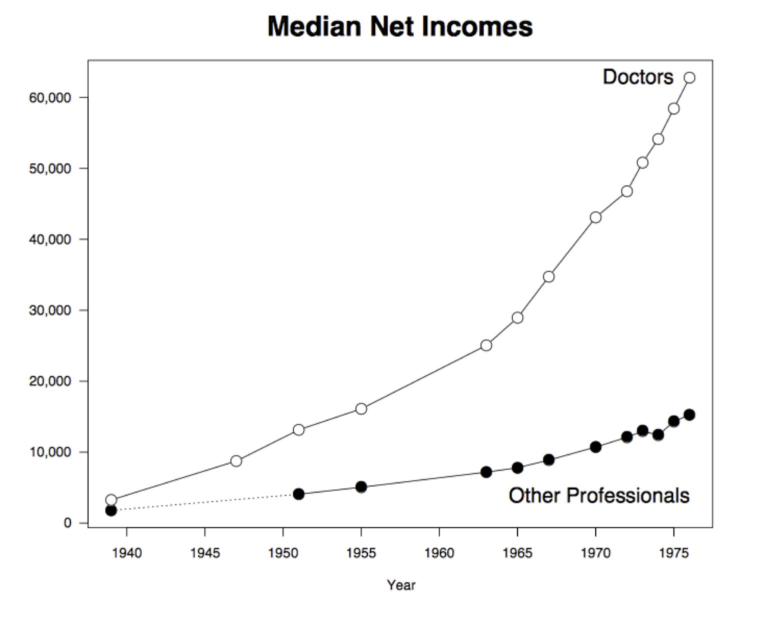
Here, from the Washington Post in the early 1980s, is a graph that attempts to compare the earnings of doctors with the earnings of other professionals over a few decades. Do we really need to see two heads (one with a stethoscope) on each bar? Tufts coined the term "chartjunk" for such unnecessary embellishments. He also deplores the "low data-to-ink ratio" which this graph unfortunately possesses.

Most importantly, the horizontal axis of the graph is is not drawn to scale. This has a significant effect on the shape of the bar graphs. When drawn to scale and shorn of decoration, the graphs reveal trends that are quite different from the apparently linear growth in the original. The elegant graph below is due to Ross Ihaka, one of the originators of the statistical system R.
Here is a graphic from Statistics Canada, a website produced by the Government of Canada.
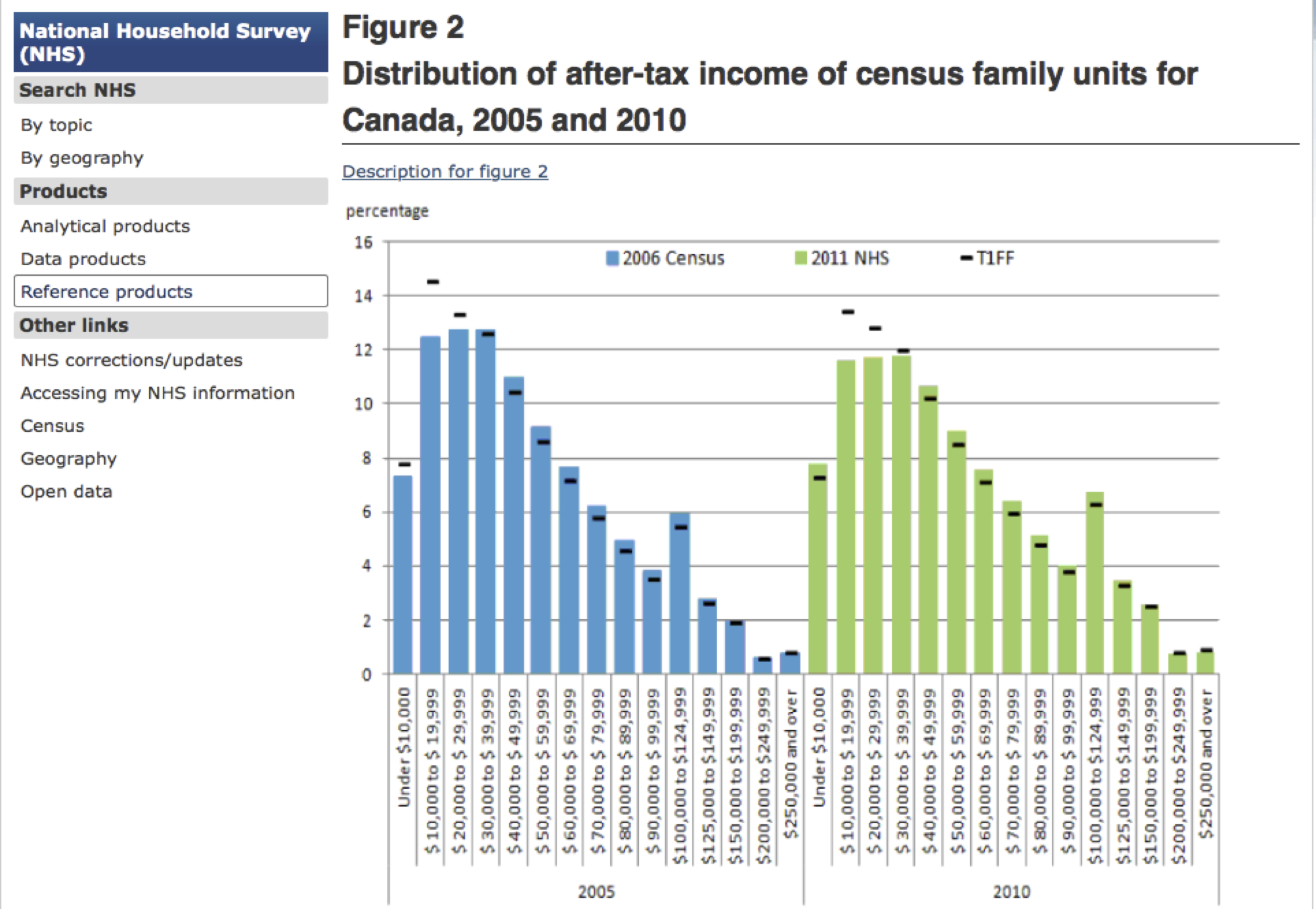
The graphs represent the distribution of after-tax income, in Canadian dollars, of families in Canada. The blue graph uses figures from the 2006 Census while the green graph shows estimates for 2010 based on the National Household Survey.
Based on what you have learned about visualization thus far, what is your assessment of this graphic?
Bar Charts and Histograms
Categorical Data and Bar Charts
Now that we have examined several graphics produced by others, it is time to produce some of our own. We will start with bar charts, a type of graph with which you might already be familiar. A bar chart shows the distribution of a categorical variable, that is, a variable whose values are categories. In human populations, examples of categorical variables include gender, ethnicity, marital status, country of citizenship, and so on.
A bar chart consists of a sequence of rectangular bars, one corresponding to each category. The length of each bar is proportional to the number of entries in the corresponding category.
We will start by drawing a bar chart of the genres of a set of movies. The data are in a table called tableA, which looks like this:
tableA
The first column of tableA is labeled GENRE. It consists of the names of various genres of movie. More formally, it contains the names of the categories of the genre variable. The second column is labeled COUNT, and contains the number of movies in each genre.
The method barh can be applied to a table with two columns as above, to produce a bar chart consisting of horizontal bars. The horizontal orientation makes it easier to label the bars. The argument that barh requires is the name of the column consisting of the categories. The length of each bar is the count in that category.
Let us apply barh to tableA, with the GENRE column as its argument.
tableA.barh('GENRE')

A different table called tableB also consists of movie genre data, in columns labled GENRE and COUNT just as in tableA. Here is a bar chart of the data in tableB.
tableB.barh('GENRE')

At first glance, it applears that the two bar charts are quite different. One of them shows a distribution that looks like a smooth curve, while the other is quite irregular. However, closer inspection reveals that the two bar charts are in fact representations of exactly the same set of data. The only difference is in the order in which the categories appear. As we have seen before with graphs that involve two axes, it is important to study both axes carefully before making conclusions.
Unlike numbers, categories do not have a unique ordering relative to each other. The user determines the order in which they appear. In tableA, the categories are arranged so that the bars appear in decreasing order of length. In tableB, the categories are listed in alphabetical order. You could randomize the order; the data would tell the same story, though some orderings might make the story a little easier to read.
The data used in the bar charts above represent the market share for each genre of Hollywood movie, from 1995 to 2015. The source is the website The Numbers, subtitled "where data and the movie business meet."
Quantitative Data and Histograms
Many of the variables that data scientists study are quantitative. These are measurements of numerical variables such as income, height, age, and so on. In keeping with the movie theme of this section, we will study the amount of money grossed by movies in recent decades. Our source is the Internet Movie Database. The IMDb is an online database that consists of a vast repository of information about movies, television shows, video games, and so on.
The table imdb consists of IMDb's data on U.S.A.'s top grossing movies of all time. The first column contains the rank of the movie; Avatar has the top rank, with a box office gross amount of more than 760 million dollars in the United States. The second column contains the name of the movie; the third contains the U.S. box office gross in dollars; and the fourth contains the same gross amount, in millions of dollars.
There are 627 movies on the list. Here are the top ten.
imdb = Table.read_table('imdb.csv')
imdb
Three-digit numbers (even with a few decimal places) are easier to work with than nine-digit numbers. So we will work with a smaller table called mill, created by selecting just the fourth column of imdb.
The method hist applied to one numerical column such as mill produces a figure called a histogram that looks very much like a bar chart. In this section, we will examine histograms and their properties.
mill = imdb.select(['in_millions'])
mill.hist()

The figure above shows the distribution of the amounts grossed, in millions of dollars. The amounts have been grouped into contiguous intervals called bins. Although in this dataset no movie grossed an amount that is exactly on the edge between two bins, it is worth noting that hist has an endpoint convention: bins include the data at their left endpoint, but not the data at their right endpoint. Sometimes, adjustments have to be made in the first or last bin, to ensure that the smallest and largest values of the variable are included. You saw an example of such an adjustment in the Census data used in the Tables section, where an age of "100" years actually meant "100 years old or older."
We can see that there are 10 bins (some bars are so low that they are hard to see), and that they all have the same width. We can also see that there the list contains no movie that grossed fewer than 100 million dollars; that is because we are considering only the top grossing movies of all time. It is a little harder to see exactly where the edges of the bins are placed. For example, it is not clear exactly where the value 200 lies on the horizontal axis, and so it is hard to judge exactly where the first bar ends and the second begins.
The optional argument bins can be used with hist to specify the edges of the bars. It must consist of a sequence of numbers that includes the left end of the first bar and the right end of the last bar. As the highest gross amount is somewhat over 760 on the horizontal scale, we will start by setting bins to be the array consisting of the numbers 100, 150, 200, 250, and so on, ending with 800.
mill.hist(bins=np.arange(100,810,50))

This figure is easier to read. On the horizontal axis, the labels 100, 200, 300, and so on are centered at the corresponding values. The number of movies that grossed between 100 million and 150 million dollars appears to be around 340; the number that grossed between 150 million and 200 million dollars appears to be around 125; and so on.
A large majority of the movies grossed between 100 million and 250 million dollars. A very small number grossed more than 600 million dollars. This results in the figure being "skewed to the right,", or, less formally, having "a long right hand tail." Distributions of variables like income or rent often have this kind of shape.
The exact counts are given below. The entries of 250 million dollars or more have been collected in a single bin. The total of the counts is 627, which is the number of movies on the list.
bins, counts = ["[100, 150)", "[150,200)", "[200, 250)", "[250, 800)"],[338,129,68,92]
bincounts = Table([bins, counts], ['bins','counts'])
bincounts
What is wrong with this picture?
Let us try to redraw the histogram with just four bins: [100, 150), [150, 200), [200, 250), and [250, 800). As we saw in the table of counts, the [250, 800) bin contains 92 movies.
mill.hist(bins=[100, 150, 200, 250, 800])

Even though the method used is called hist, the figure above is NOT A HISTOGRAM. It gives the impression that there are many more movies in the 250-800 bin than in the 100-150 bin, and indeed more than in the entire range 100-250. The height of each bar is simply plotted the number of movies in the bin, without accounting for the difference in the widths of the bins.
So what is a histogram?
The figure above shows that what the eye perceives as "big" is area, not just height. This is particularly important when the bins are of different widths.
That is why a histogram has two defining properties:
- The bins are contiguous (though some might be empty) and are drawn to scale.
- The area of each bar is proportional to the number of entries in the bin.
Property 2 is the key to drawing a histogram, and is usually achieved as follows:
$$ \mbox{area of bar} ~=~ \mbox{proportion of entries in bin} $$When drawn using this method, the histogram is said to be drawn on the density scale, and the total area of the bars is equal to 1.
To calculate the height of each bar, use the fact that the bar is a rectangle:
$$ \mbox{area of bar} = \mbox{height of bar} \times \mbox{width of bin} $$and so
$$ \mbox{height of bar} ~=~ \frac{\mbox{area of bar}}{\mbox{width of bin}} ~=~ \frac{\mbox{proportion of entries in bin}}{\mbox{width of bin}} $$For hist to draw a histogram on the density scale, the Boolean option normed must have the value True. You can think of "normed" as shorthand for "follows the norm of the density scale."
mill.hist(bins=[100, 150, 200, 250, 800], normed=True)

This is a reasonable representation of the data, though of course some detail has been lost. The level of detail in a histogram depends on the level of detail in the data as well as on the choices made by the user. Before we explore this idea further, let us first check that the numbers on the vertical axis above are consistent with the heights that we would calculate.
There are 129 movies in the [150, 200) bin. The proportion of movies in the bin is therefore 129/627, and the width of the bin is 200-150. So the height of the bar above that bin should be
$$ \frac{129/627}{200-150} ~=~ 0.0041148325358851675 $$That agrees with the height of the bar as shown in the figure. You might want to check that the other heights also agree with what you would calculate.
The level of detail, and the flat tops of the bars
Take another look at the [150, 200) bin in the figure above. The flat top of the bar, at the level 0.004, hides the fact that the movies are somewhat unevenly distributed across the bin. To see this, let us split the [150, 200) bin into five narrower bins of width 10 million dollars each:
mill.hist(bins=[100, 150, 160, 170, 180, 190, 200, 250, 800], normed=True)

Some of the skinny bars are taller than 0.004 and others are shorter. By putting a flat top at 0.004 over the whole bin, we are deciding to ignore the finer detail and use the flat level as a rough approximation. Often, though not always, this is sufficient for understanding the general shape of the distribution.
Notice that because we have the entire dataset, we can draw the histogram in as fine a level of detail as the data and our patience will allow. However, if you are looking at a histogram in a book or on a website, and you don't have access to the underlying dataset, then it becomes important to have a clear understanding of the "rough approximation" of the flat tops.
The density scale
The height of each bar is a proportion divided by a bin width. Thus, for this datset, the values on the vertical axis are "proportions per million dollars." To understand this better, look again at the [150, 200) bin. The bin is 50 million dollars wide. So we can think of it as consisting of 50 narrow bins that are each 1 million dollars wide. The bar's height of roughly "0.004 per million dollars" means that in each of those 50 skinny bins of width 1 million dollars, the proportion of movies is roughly 0.004.
Thus the height of a histogram bar is a proportion per unit on the horizontal axis, and can be thought of as the density of entries per unit width.
imdb.select(['in_millions']).hist(bins=[100, 150, 200, 250, 800], normed=True)
Density Q&A
Look again at the histogram, and this time compare the [200, 250) bin with the [250, 800) bin.
Q: Which has more movies in it?
A: The [250, 800) bin. It has 92 movies, compared with 68 movies in the [200, 250) bin.
Q: Then why is the [250, 800) bar shorter than the [200, 250) bar?
A: Because height represents density per unit width, not the number of movies in the bin. The [250, 800) bin has more movies than the [200, 250) bin, but it is also a whole lot wider. So the density is much lower.
Bar chart or histogram?
Bar charts display the distributions of categorical variables. All the bars in a bar chart have the same width. The lengths (or heights, if the bars are drawn vertically) of the bars are proportional to the number of entries.
Histograms display the distributions of quantitative variables. The bars can have different widths. The areas of the bars are proportional to the number of entries.
Multiple bar charts and histograms
In all the examples in this section, we have drawn a single bar chart or a single histogram. However, if a data table contains several columns, then barh and hist can be used to draw several graphs at once. We will cover this feature in a later section.
Functions
We are building up a useful inventory of techniques for identifying patterns and themes in a data set. Sorting and filtering rows of a table can focus our attention. Bar charts and histograms can summarize data visually to convey broad numerical patterns. The next approach to analysis we will consider involves grouping rows of a table by arbitrary criteria. To do so, we will explore two core features of the Python programming language: function definition and conditional statements.
We have used functions extensively already in this text, but never defined a function of our own. The purpose of defining a function is to give a name to a computational process that may be applied multiple times. Although there are many situations in computing that require repeating a computational process many times, the most natural one in our setting is to perform the same process on each row of a table.
A function is defined in Python using a def statement, which is a multi-line
statement that begins with a header line giving the name of the function and
names for the arguments of the function. The rest of the def statement,
called the body, must be indented below the header.
A function expresses a relationship between its inputs (called arguments) and
its outputs (called return values). The number of arguments required to call
a function is the number of names that appear within parentheses in the def
statement header. The values that are returned depend on the body. Whenever a
function is called, its body is executed. Whenever a return statement within
the body is executed, the call to the function completes and the value of the
expression directly following return is returned.
The definition of the percent function below multiplies a number by 10 and rounds the result to two decimal places.
def percent(x):
    return round(100*x, 2)
The primary difference between defining a percent function and simply evaluating its return expression round(100*x, 2) is that when a function is defined, its return expression is not immediately evaluated. It cannot be, because the value for x is not yet defined. Instead, the return expression is evaluated whenever this percent function is called by placing parentheses after the name percent and placing an expression to compute its argument in parentheses.
percent(1/6)
percent(1/6000)
percent(1/60000)
In the expression above, called a call expression, the value of 1/6 is computed and then passed as the argument named x to the percent function. When the percent function is called in this way, its body is executed. The body of percent has only a single line: return round(100*x, 2). Executing this return statement completes execution of the percent function's body and gives the value of the call expression percent(1/6).
The same result is computed by passing a named value as an argument. The percent function does not know or care how its argument is computed; its only job is to execute its own body using the argument names that appear in its header.
sixth = 1/6
percent(sixth)
Conditional Statements. The body of a function can have more than one line and more than one return statement. A conditional statement is a multi-line statement that allows Python to choose among different alternatives based on the truth value of an expression. While conditional statements can appear anywhere, they appear most often within the body of a function in order to express alternative behavior depending on argument values.
A conditional statement always begins with an if header, which is a single line followed by an indented body. The body is only executed if the expression directly following if (called the if expression) evaluates to a true value. If the if expression evaluates to a false value, then execution of the function body continues.
For example, we can improve our percent function so that it doesn't round very small numbers to zero so readily. The behavior of percent(1/6) is unchanged, but percent(1/60000) provides a more useful result.
def percent(x):
    if x < 0.00005:
        return 100 * x
    return round(100 * x, 2)
percent(1/6)
percent(1/6000)
percent(1/60000)
A conditional statement can also have multiple clauses with multiple bodies, and only one of those bodies can ever be executed. The general format of a multi-clause conditional statement appears below.
if <if expression>:
    <if body>
elif <elif expression 0>:
    <elif body 0>
elif <elif expression 1>:
    <elif body 1>
...
else:
    <else body>
There is always exactly one if clause, but there can be any number of elif clauses. Python will evaluate the if and elif expressions in the headers in order until one is found that is a true value, then execute the corresponding body. The else clause is optional. When an else header is provided, its else body is executed only if none of the header expressions of the previous clauses are true. The else clause must always come at the end (or not at all).
Let us continue to refine our percent function. Perhaps for some analysis, any value below $10^{-8}$ should be considered close enough to 0 that it can be ignored. The following function definition handles this case as well.
def percent(x):
    if x < 1e-8:
        return 0.0
    elif x < 0.00005:
        return 100 * x
    else:
        return round(100 * x, 2)
percent(1/6)
percent(1/6000)
percent(1/60000)
percent(1/60000000000)
A well-composed function has a name that evokes its behavior, as well as a docstring — a description of its behavior and expectations about its arguments. The docstring can also show example calls to the function, where the call is preceded by >>>.
A docstring can be any string that immediately follows the header line of a def statement. Docstrings are typically defined using triple quotation marks at the start and end, which allows the string to span multiple lines. The first line is conventionally a complete but short description of the function, while following lines provide further guidance to future users of the function.
A more complete definition of percent that includes a docstring appears below.
def percent(x):
    """Convert x to a percentage by multiplying by 100.

    Percentages are conventionally rounded to two decimal places,
    but precision is retained for any x above 1e-8 that would
    otherwise round to 0.

    >>> percent(1/6)
    16.67
    >>> perent(1/6000)
    0.02
    >>> perent(1/60000)
    0.0016666666666666668
    >>> percent(1/60000000000)
    0.0
    """
    if x < 1e-8:
        return 0.0
    elif x < 0.00005:
        return 100 * x
    else:
        return round(100 * x, 2)
Functions and Tables
In this section, we will continue to use the imdb.csv data set.
imdb = Table.read_table('imdb.csv')
Functions can be used to compute new columns in a table based on existing column values. For example, the IMDb dataset of top grossing movies placed the year of each movie in the title. To categorize the data by year, we first must separate the title from the date.
Slicing. Titles are strings, and a string is a sequence. Any sequence can be sliced, creating a new sequence of the same type that has only a range of the original elements. To slice a sequence, place two indices separated by a colon within square brackets. While slicing has a new syntax, slices have the same behavior as the arguments to np.arange: the first number is an inclusive lower bound and the second argument is an exclusive upper bound.
title = "Terminator 2: Judgment Day (1991)"
title[3:10]
Negative indices in a slice (or in element selection) count from the end of the sequence. Since years of movies in this data set always contain exactly 4 numbers, we can separate the date from the title using a slice and negative constants.
title[-5:-1]
The year function below takes in a movie title with the year at the end, slices out the year, and converts the result to an integer by calling int.
def year(title):
    """Return the year of a movie, assuming it appears at the end of the title."""
    return int(title[-5:-1])

year(title)
Apply. The apply method of a table calls a function on each element of a column, forming a new array of return values. To indicate which function to call, just name it (without quotation marks). The name of the column of input values must still appear within quotation marks.
imdb['year'] = imdb.apply(year, 'movie')
imdb
Computing Categories
Functions can also be used to create categories based on existing columns. The first step in categorizing data is to write a function that can take existing column values as arguments and return a category label. Then, a new column for that category can be added using apply, as in the example above.
Certain science fiction films have pushed the limits of special effects technology. The movie E.T., released in 1982, made audiences believe in aliens. Jurassic Park, released in 1993, delivered the most convincing images of dinosaurs ever created. Avatar, released in 2009, created realistic humanoid aliens in immersive 3-dimensional films. We can use these landmarks of special effects technology to categorize the history of cinema.
def age(year):
    if year < 1982:
        return 'old'
    elif year < 1993:
        return 'modern'
    elif year < 2009:
        return 'recent'
    else:
        return 'contemporary'

imdb['era'] = imdb.apply(age, 'year')
imdb
Once a new category column is introduced, it can be used to perform any sort of further processing. For instance, we could count how many movies come from each era.
imdb.select(['era', 'year']).group('era', len).barh('era')

Functions can also be used to generate visualizations from tables. Histograms of the eras show quite a contrast in the distribution of movie proceeds over the years. What changes might explain the trend you observe? How might you investigate whether that change accounts for the trend?
def age_hist(age):
    imdb.where('era', age).select(['in_millions']).hist(
        bins=np.arange(100, 1000, 50),
        normed=True)

age_hist('old')
age_hist('modern')
age_hist('recent')
age_hist('contemporary')


Sampling
In this section, we will continue to use the imdb.csv data set.
imdb = Table.read_table('imdb.csv')
Sampling rows of a table
Deterministic Samples
When you simply specify which elements of a set you want to choose, without any chances involved, you create a deterministic sample.
A determinsitic sample from the rows of a table can be constructed using the take method. Its argument is a sequence of integers, and it returns a table containing the corresponding rows of the original table.
The code below returns a table consisting of the rows indexed 3, 18, and 100 in the table imdb. Since the original table is sorted by rank, which begins at 1, the zero-indexed rows always have a rank that is one greater than the index. However, the take method does not inspect the information in the rows to construct its sample.
imdb.take([3, 18, 100])
We can select evenly spaced rows by calling np.arange and passing the result to take. In the example below, we start with the first row (index 0) of imdb, and choose every 100th row after that until we reach the end of the table. The expressions imdb.num_rows and len(imdb.rows) could be used interchangeably to indicate that the range should extend to the end of the table.
imdb.take(np.arange(0, imdb.num_rows, 100))
Probability Samples
Much of data science consists of making conclusions based on the data in random samples. Correctly interpreting analyses based on random samples requires data scientists to examine exactly what random samples are.
A population is the set of all elements from whom a sample will be drawn.
A probability sample is one for which it is possible to calculate, before the sample is drawn, the chance with which any subset of elements will enter the sample.
In a probability sample, all elements need not have the same chance of being chosen. For example, suppose you choose two people from a population that consists of three people A, B, and C, according to the following scheme:
- Person A is chosen with probability 1.
- One of Persons B or C is chosen according to the toss of a coin: if the coin lands heads, you choose B, and if it lands tails you choose C.
This is a probability sample of size 2. Here are the chances of entry for all non-empty subsets:
A: 1
B: 1/2
C: 1/2
AB: 1/2
AC: 1/2
BC: 0
ABC: 0
Person A has a higher chance of being selected than Persons B or C; indeed, Person A is certain to be selected. Since these differences are known and quantified, they can be taken into account when working with the sample.
To draw a probability sample, we need to be able to choose elements according to a process that involves chance. A basic tool for this purpose is a random number generator. There are several in Python. Here we will use one that is part of the module random, which in turn is part of the module numpy.
The method randint, when given two arguments low and high, returns an integer picked uniformly at random between low and high, including low but excluding high. Run the code below several times to see the variability in the integers that are returned.
np.random.randint(3, 8) # select once at random from 3, 4, 5, 6, 7
A Systematic Sample
Imagine all the elements of the population listed in a sequence. One method of sampling starts by choosing a random position early in the list, and then evenly spaced positions after that. The sample consists of the elements in those positions. Such a sample is called a systematic sample.
Here we will choose a systematic sample of the rows of imdb. We will start by picking one of the first 10 rows at random, and then we will pick every 10th row after that.
"""Choose a random start among rows 0 through 9;
then take every 10th row."""

start = np.random.randint(0, 10)
imdb.take(np.arange(start, imdb.num_rows, 10))
Run the code a few times to see how the output varies. Notice how the numbers in the rank column all have the same ending digit. That is because the first row has a random index between 0 and 9, and hence a random rank between 1 and 10; then the code just adds 10 successively to each selected row index, leaving the ending digit unchanged.
This systematic sample is a probability sample. To find the chance that a particular row is selected, look at the ending digit in the rank column of the row. If that is 7, for example, then the row will be selected if and only if the row corresponding to movie rank 7 (Star Wars) is selected. The chance of that is 1/10.
In this scheme, all rows do have the same chance of being chosen. But that is not true of other subsets of the rows. Because the selected rows are evenly spaced, most subsets of rows have no chance of being chosen. The only subsets that are possible are those in which all the ranks have the same ending digit. Those are selected with chance 1/10.
Random sample with replacement
Some of the simplest probability samples are formed by drawing repeatedly, uniformly at random, from the list of elements of the population. If the draws are made without changing the list between draws, the sample is called a random sample with replacement. You can imagine making the first draw at random, replacing the element drawn, and then drawing again.
In a random sample with replacement, each element in the population has the same chance of being drawn, and each can be drawn more than once in the sample.
If you want to draw a sample of people at random to get some information about a population, you might not want to sample with replacement – drawing the same person more than once can lead to a loss of information. But in data science, random samples with replacement arise in two major areas:
studying probabilities by simulating tosses of a coin, rolls of a die, or gambling games
creating new samples from a sample at hand
The second of these areas will be covered later in the course. For now, let us study some long-run properties of probabilities.
We will start with the table die which contains the numbers of spots on the faces of a die. All the numbers appear exactly once, as we are assuming that the die is fair.
die = Table([[1, 2, 3, 4, 5, 6]],['Face'])
die
Drawing the histogram of this simple set of numbers yields an unsettling figure as hist makes a default choice of bins:
die.hist()

The numbers 1, 2, 3, 4, 5, 6 are integers, so the bins chosen by hist only have entries at the edges. In such a situation, it is a better idea to select bins so that they are centered on the integers. This is often true of histograms of data that are discrete, that is, variables whose successive values are separated by the same fixed amount. The real advantage of this method of bin selection will become more clear when we start imagining smooth curves drawn over histograms.
die.hist(bins=np.arange(0.5, 7, 1), normed=True)

Notice how each bin has width 1 and is centered on an integer. Notice also that because the width of each bin is 1, the height of each bar is $0.16666 \ldots /1 = 1/6$, the chance that the corresponding face appears.
The histogram shows the probability with which each face appears. It is called a probability histogram of the result of one roll of a die.
The histogram was drawn without rolling any dice or generating any random numbers. We will now use the computer to mimic actually rolling a die. The process of using a computer program to produce the results of a chance experiment is called simulation.
To roll the die, we will use a method called sample. This method returns a new table consisting of rows selected uniformly at random from a table. Its first argument is the number of rows to be returned. Its second argument is whether or not the sampling should be done with replacement.
The code below simulates 10 rolls of the die. As with all simulations of chance experiments, you should run the code several times and notice the variability in what is returned.
die.sample(10, with_replacement=True)
We will now roll the die several times and draw the histogram of the observed results. The histogram of observed results is called an empirical histogram.
The results of rolling the die will all be integers in the range 1 through 6, so we will want to use the same bins as we used for the probability histogram. To avoid writing out the same bin argument every time we draw a histogram, let us define a function called hist_1to6 that will perform the task for us. The function will take one argument: the name of a table that contains the results of the rolls.
def hist_1to6(x):
    return x.hist(bins=np.arange(0.5, 7, 1), normed=True)
hist_1to6(die.sample(20, with_replacement=True))

Below, for comparison, is the probability histogram for the roll of a die. Based on that, we expect each face to appear about on $1/6$ of the rolls. But if you run the simulation above a few times, you will see that with just 20 rolls, the proportion of times each face appears can be quite far from $1/6$.
hist_1to6(die)
As we increase the number of rolls in the simulation, the proportions get closer to $1/6$.
hist_1to6(die.sample(2000, with_replacement=True))

The behavior we have observed is an instance of a general rule.
The Law of Averages
If a chance experiment is repeated independently and under identical conditions, then, in the long run, the proportion of times that an event occurs gets closer and closer to the theoretical probability of the event.
For example, in the long run, the proportion of times the face with four spots appears gets closer and closer to 1/6.
Here "independently and under identical conditions" means that every repetition is performed in the same way regardless of the results of all the other repetitions.
Convergence of empirical histograms
We have also observed that a random quantity (such as the number of spots on one roll of a die) is associated with two histograms:
a probability histogram, that shows all the possible values of the quantity and all their chances
an empirial histogram, created by simulating the random quantity repeatedly and drawing a histogram of the observed results
We have seen an example of the long-run behavior of empirical histograms:
As the number of repetitions increases, the empirical histogram of a random quantity looks more and more like the probability histogram.
At the Roulette Table
Equipped with our new knowledge about the long-run behavior of chances, let us explore a gambling game. Betting on roulette is popular in gambling centers such as Las Vegas and Monte Carlo, and we will simulate one of the bets here.
The main randomizer in roulette in Nevada is a wheel that has 38 pockets on its rim. Two of the pockets are green, eighteen black, and eighteen red. The wheel is on a spindle, and there is a small ball on it. When the wheel is spun, the ball ricochets around and finally comes to rest in one of the pockets. That is declared to be the winning pocket.
You are allowed to bet on several pre-specified collections of pockets. If you bet on "red," you win if the ball comes to rest in one of the red pockets.
The bet even money. That is, it pays 1 to 1. To understand what that means, assume you are going to bet \$1 on "red." The first thing that happens, even before the wheel is spun, is that you have to hand over your \$1. If the ball lands in a green or black pocket, you never see that dollar again. If the ball lands in a red pocket, you get your dollar back (to bring you back to even), plus another \$1 in winnings.
The table wheel represents the pockets of a Nevada roulette wheel. It has 38 rows labeled 1 through 38, one row per pocket.
pockets = np.arange(1, 39)
colors = (['red', 'black'] * 5 + ['black', 'red'] * 4) * 2 + ['green', 'green']
wheel = Table([pockets, colors],['pocket', 'color'])
wheel
The function bet_on_red takes a numerical argument x and returns the net winnings on a \$1 bet on "red," provided x is the number of a pocket.
def bet_on_red(x):
    """The net winnings of betting on red for outcome x."""
    pockets = wheel.where('pocket', x)
    if pockets['color'][0] == 'red':
        return 1
    else:
        return -1
bet_on_red(17)
The function spins takes a numerical argument n and returns a new table consisting of n rows of wheel sampled at random with replacement. In other words, it simulates the results of n spins of the roulette wheel.
def spins(n):
    return wheel.sample(n, with_replacement=True)
We will create a table called play consisting of the results of 10 spins, and add a column that shows the net winnings on \$1 placed on "red." Recall that the apply method applies a function to each element in a column of a table.
play = spins(10)
play['winnings'] = play.apply(bet_on_red, 'pocket')
play
And here is the net gain on all 10 bets:
sum(play['winnings'])
We can put all this together in a single function called fate_red that takes as its argument the number of bets and returns the net gain on that many \$1 bets placed on "red." Try running fate_red several times with an argument of 500.
def fate_red(n):
    net_gain = sum(spins(n).apply(bet_on_red, 'pocket'))
    if net_gain > 0:
        return 'You made ' + str(net_gain) + " dollars. Lucky!"
    elif net_gain == 0:
        return "Whew! Broke even."
    elif net_gain < 0:
        return 'You made '+ str(net_gain) + " dollars. The casino thanks you for making it richer."
fate_red(500)
Betting \$1 on red hundreds of times seems like a bad idea from a gambler's perspective. But from the casinos' perspective it is excellent. Casinos rely on large numbers of bets being placed. The payoff odds are set so that the more bets that are placed, the more money the casinos are likely to make, even though a few people are likely to go home with winnings.
Simple Random Sample – a Random Sample without Replacement
A random sample without replacement is one in which elements are drawn from a list repeatedly, uniformly at random, at each stage deleting from the list the element that was drawn.
A random sample without replacement is also called a simple random sample. All elements of the population have the same chance of entering a simple random sample. All pairs have the same chance as each other, as do all triples, and so on.
The default action of sample is to draw without replacement. In card games, cards are almost always dealt without replacement. Let us use sample to deal cards from a deck.
A standard deck deck consists of 13 ranks of cards in each of four suits. The suits are called spades, clubs, diamonds, and hearts. The ranks are Ace, 2, 3, 4, 5, 6, 7, 8, 9, 10, Jack, Queen, and King. Spades and clubs are black; diamonds and hearts are red. The Jacks, Queens, and Kings are called 'face cards.'
The table deck contains all 52 cards in a column labeled cards. The abbreviations are:
Spades: s $~~$ Clubs: c $~~$ Diamonds: d $~~$ Hearts: h
Ace: A $~~$ Jack: J $~~$ Queen: Q $~~$ King: K
from itertools import product

suits = ['♠︎', '♥︎', '♦︎', '♣︎']
ranks = ['A', '2', '3', '4', '5', '6', '7', '8', '9', '10', 'J', 'Q', 'K']

deck = Table.from_rows(product(ranks, suits), ['rank', 'suit'])
deck
A poker hand is five cards dealt at random from the deck. The code below deals a poker hand. Deal a few hands to see if you can get a flush: a hand that contains only one suit. How many aces do you typically get?
deck.sample(5)
Note that the hand is the set of five cards, regardless of the order in which they appeared. For example, the hand ['9♣︎', '9♥︎', 'Q♣︎', '7♣︎', '8♥︎'] is the same as the hand ['7♣︎', '9♣︎', '8♥︎', '9♥︎', 'Q♣︎'].
This can be used to show that simple random sampling can be thought of in two equivalent ways:
drawing elements one by one at random without replacement
randomly permuting (that is, shuffling) the whole list, and then pulling out a set of elements at the same time
Explorations: Privacy
License plates
We're going to look at some data collected by the Oakland Police Department. They have automated license plate readers on their police cars, and they've built up a database of license plates that they've seen -- and where and when they saw each one.
Data collection
First, we'll gather the data. It turns out the data is publicly available on the Oakland public records site. I downloaded it and combined it into a single CSV file by myself before lecture.
lprs = Table.read_table('./all-lprs.csv.gz', compression='gzip', sep=',')
lprs.column_labels
Let's start by renaming some columns, and then take a look at it.
lprs.relabel('red_VRM', 'Plate')
lprs.relabel('red_Timestamp', 'Timestamp')
lprs
Phew, that's a lot of data: we can see about 2.7 million license plate reads here.
Let's start by seeing what can be learned about someone, using this data -- assuming you know their license plate.
Stalking Jean Quan
As a warmup, we'll take a look at ex-Mayor Jean Quan's car, and where it has been seen. Her license plate number is 6FCH845. (How did I learn that? Turns out she was in the news for getting $1000 of parking tickets, and the news article included a picture of her car, with the license plate visible. You'd be amazed by what's out there on the Internet...)
lprs.where('Plate', '6FCH845')
OK, so her car shows up 6 times in this data set. However, it's hard to make sense of those coordinates. I don't know about you, but I can't read GPS so well.
So, let's work out a way to show where her car has been seen on a map. We'll need to extract the latitude and longitude, as the data isn't quite in the format that the mapping software expects: the mapping software expects the latitude to be in one column and the longitude in another. Let's write some Python code to do that, by splitting the Location string into two pieces: the stuff before the comma (the latitude) and the stuff after (the longitude).
def getlatitude(s):
    before, after = s.split(',') # Break it into two parts
    latstring = before[1:] # Get rid of the annoying '('
    return float(latstring) # Convert the string to a number
def getlongitude(s):
    before, after = s.split(',') # Break it into two parts
    longstring = after[1:-1] # Get rid of the ' ' and the ')'
    return float(longstring) # Convert the string to a number
Let's test it to make sure it works correctly.
getlatitude('(37.797558, -122.26935)')
getlongitude('(37.797558, -122.26935)')
Good, now we're ready to add these as extra columns to the table.
lprs['Latitude'] = lprs.apply(getlatitude, 'Location')
lprs['Longitude'] = lprs.apply(getlongitude, 'Location')
lprs = lprs.drop('Location')
lprs
And at last, we can draw a map with a marker everywhere that her car has been seen.
jeanquan = lprs.where('Plate', '6FCH845')
Marker.map(jeanquan['Latitude'], jeanquan['Longitude'], labels=jeanquan['Timestamp'])
OK, so it's been seen near the Oakland police department. This should make you suspect we might be getting a bit of a biased sample. Why might the Oakland PD be the most common place where her car is seen? Can you come up with a plausible explanation for this?
Poking around
Let's try another. And let's see if we can make the map a little more fancy. It'd be nice to distinguish between license plate reads that are seen during the daytime (on a weekday), vs the evening (on a weekday), vs on a weekend. So we'll color-code the markers. To do this, we'll write some Python code to analyze the Timestamp and choose an appropriate color.
import datetime
def getcolor(ts):
    t = datetime.datetime.strptime(ts, '%m/%d/%Y %I:%M:%S %p')
    if t.weekday() >= 6:
        return 'green' # Weekend
    if t.hour >= 6 and t.hour <= 17:
        return 'blue' # Weekday daytime
    return 'red' # Weekday evening
lprs['Color'] = lprs.apply(getcolor, 'Timestamp')
Now we can check out another license plate, this time with our spiffy color-coding. This one happens to be the car that the city issues to the Fire Chief.
t = lprs.where('Plate', '1328354')
Marker.map(t['Latitude'], t['Longitude'], labels=t['Timestamp'], colors=t['Color'])
Hmm. We can see a blue cluster in downtown Oakland, where the Fire Chief's car was seen on weekdays during business hours. I bet we've found her office. In fact, if you happen to know downtown Oakland, those are mostly clustered right near City Hall. Also, her car was seen twice in northern Oakland on weekday evenings. One can only speculate what that indicates. Maybe dinner with a friend? Or running errands? Off to the scene of a fire? Who knows. And then the car has been seen once more, late at night on a weekend, in a residential area in the hills. Her home address, maybe?
Let's look at another.
t = lprs.where('Plate', '5AJG153')
Marker.map(t['Latitude'], t['Longitude'], labels=t['Timestamp'], colors=t['Color'])
What can we tell from this? Looks to me like this person lives on International Blvd and 9th, roughly. On weekdays they've seen in a variety of locations in west Oakland. It's fun to imagine what this might indicate -- delivery person? taxi driver? someone running errands all over the place in west Oakland?
We can look at another:
t = lprs.where('Plate', '6UZA652')
Marker.map(t['Latitude'], t['Longitude'], labels=t['Timestamp'], colors=t['Color'])
What can we learn from this map? First, it's pretty easy to guess where this person lives: 16th and International, or pretty near there. And then we can see them spending some nights and a weekend near Laney College. Did they have an apartment there briefly? A relationship with someone who lived there?
Is anyone else getting a little bit creeped out about this? I think I've had enough of looking at individual people's data.
Inference
As we can see, this kind of data can potentially reveal a fair bit about people. Someone with access to the data can draw inferences. Take a moment to think about what someone might be able to infer from this kind of data.
As we've seen here, it's not too hard to make a pretty good guess at roughly where some lives, from this kind of information: their car is probably parked near their home most nights. Also, it will often be possible to guess where someone works: if they commute into work by car, then on weekdays during business hours, their car is probably parked near their office, so we'll see a clear cluster that indicates where they work.
But it doesn't stop there. If we have enough data, it might also be possible to get a sense of what they like to do during their downtime (do they spend time at the park?). And in some cases the data might reveal that someone is in a relationship and spending nights at someone else's house. That's arguably pretty sensitive stuff.
This gets at one of the challenges with privacy. Data that's collected for one purpose (fighting crime, or something like that) can potentially reveal a lot more. It can allow the owner of the data to draw inferences -- sometimes about things that people would prefer to keep private. And that means that, in a world of "big data", if we're not careful, privacy can be collateral damage.
Mitigation
If we want to protect people's privacy, what can be done about this? That's a lengthy subject. But at risk of over-simplifying, there are a few simple strategies that data owners can take:
Minimize the data they have. Collect only what they need, and delete it after it's not needed.
Control who has access to the sensitive data. Perhaps only a handful of trusted insiders need access; if so, then one can lock down the data so only they have access to it. One can also log all access, to deter misuse.
Anonymize the data, so it can't be linked back to the individual who it is about. Unfortunately, this is often harder than it sounds.
Engage with stakeholders. Provide transparency, to try to avoid people being taken by surprise. Give individuals a way to see what data has been collected about them. Give people a way to opt out and have their data be deleted, if they wish. Engage in a discussion about values, and tell people what steps you are taking to protect them from unwanted consequences.
This only scratches the surface of the subject. My main goal in this lecture was to make you aware of privacy concerns, so that if you are ever a steward of a large data set, you can think about how to protect people's data and use it responsibly.
Appendix: Statements
0. Introduction
In this note, we'll go over the structure of Python code in a bit more detail than we have before. When you've absorbed this material, you should be able to read Python code and decompose it into simple, understandable parts. This note should be particularly useful if you've seen a lot of Python code, but you have a hard time interpreting complicated-looking code like table['foo'] = np.array([1,2,3]) + table['bar'].
Decomposing Python into small parts is kind of like diagramming an English sentence. While our brains are perfectly capable of generating and understanding English without explicitly identifying things like subjects and predicates, Python interprets code very literally according to its rules (its syntax). So if you want to understand Python code, it's more important to have a precise model of Python's rules in your head. On the flip side, Python's rules are much simpler than those of English (see, for example, this amusingly complicated English sentence). They just seem complicated because we're less familiar with them. That makes it possible to learn Python much faster than you learned English.
Note: Everything in this note is also available, with even more pedantic precision, at the official Python language reference. This note is focused on the material in chapters 6, 7, and 8 of the reference. We will omit some details and fudge some truths in the interest of pedagogy. Once you feel like an expert in this stuff, feel free to brave the official documentation.
How to read this document
This note contains a bunch of code cells, in addition to text. The code cells typically illustrate points from the text. Please run the code cells as you go through the note, and pay attention to what their output is. Recall that the thing that's printed when you run a cell is the value of the last line.
1. Code is a sequence of statements
Below is a cell containing various Python code that might look familiar by now.
3                                               # Line 1.0
z = 3                                           # Line 1.1
4+3                                             # Line 1.2
y = 4+3                                         # Line 1.3
(2+3)+z                                         # Line 1.4
"foo"+"bar"                                     # Line 1.5
[1,2,3]                                         # Line 1.6
x = [1,2,3]                                     # Line 1.7
sum(x)                                          # Line 1.8
x[2]                                            # Line 1.9
x[2] = 4                                        # Line 1.10
t = Table()                                     # Line 1.11
t['Things'] = np.array(["foo", "bar", "baz"])   # Line 1.12
t.sort('Things')                                # Line 1.13
u = t.sort('Things')                            # Line 1.14
u.relabel('Things', 'Nonsense')                 # Line 1.15
u                                               # Line 1.16
(The # Line X comments are just there for labeling; don't consider them part of the lines. Similarly, other instances of # some text here that you see in this note are just for explanation.) Each line in the cell is a statement. A statement is a (somewhat) self-contained piece of code. Python executes statements in the order in which they appear. There are many kinds of statements, and to execute a statement, Python first has to figure out what kind of statement it is.
2. Expressions
The most basic kind of statement is the expression.
Line 0 above is just an expression: 3. Like many (but not all) expressions, it has a value, the integer 3. Like some (but not all) expressions, computing its value causes nothing to "happen" to the world. (We say it has no side effects.) When Python executes line 0, it computes that value. Since nothing is done with it, it just gets discarded. The same is true of lines 2, 4, 5, 6, 8, 9, 13, and 16 -- those are expression statements that cause values to be computed, but the computation has no side effects, and the value of the full expression is eventually discarded. Line 15 is an expression that does have side effects -- it causes the 'Things' column in the table named t to be renamed to 'Nonsense'. The other lines are statements but not expressions, but we will see that, like many statements, they contain expressions.
Expressions are themselves usually made up of several smaller expressions joined together by some rules; we call these compound expressions, and we sometimes call the component expressions subexpressions. Line 2, for example, is a compound expression made up of the subexpressions 4 and 3 joined by +. Python knows what a + between two expressions means, and it puts them together so that the value of 4+3 is the value of 4 plus the value of 3, or 7.
Line 4 is another compound expression. We can think of it as the subexpressions (2+3) and z, again joined by +. But (2+3) is itself a compound expression, made up of 2 and 3 joined by +. Python first computes the value of (2+3), which is 5, and then computes the value of z, which is 3 (z having been assigned previously), and then adds 5 and 3 to get 8. (2+3)*(4*((5*6)+7)) is also a valid expression. It contains 10 subexpressions (not including itself):
23(2+3)456(5*6)7((5*6)+7)(4*((5*6)+7))
Compound expressions can be arbitrarily complicated compositions of expressions.
Question. How many subexpressions are contained in the expression ((1+2)+(3+4))+((5+6)+(7+8))?
It's critical to recognize that subexpressions are valid expressions that could be written by themselves or made part of other compound expressions. If you see a complicated expression like the one above (or even more exotic ones later), and you don't understand what it does, you can always break it down into smaller bits until you get to very basic expressions. There is a fairly small list of basic expression types (things that can't be broken down into subexpressions) to learn.
This note will tell you the rules about most of the basic expressions in Python, but in order to understand and write real code (which very regularly involves large compound expressions) you'll need to develop the skill of breaking down compound expressions into subexpressions. You can try to do that mentally while you're reading code, but if that's too hard, you can just type them into a Python code cell and see what they do.
Question. What's the value of each subexpression you found above? You can just type them into the empty code cell below if you like.
A note on errors
Line 5 ("foo"+"bar") is a compound expression adding two strings, with "foo" and "bar" as subexpressions. This is okay, since the + operator knows how to handle two strings. It produces the string "foobar" as its value.
When the following cell is executed, however, there is an error. (Run the cell to confirm that.)
"foo"+5 # Error!
When you see an error, don't just give up. Often (though unfortunately not always) the error message will tell you what's wrong. The error message first tells us that the problem happened on line 1 of the cell (in this case, the only line) and the text of the error is "TypeError: Can't convert 'int' object to str implicitly". Python evaluates "foo" and 5 just fine, but when the + operator tries to apply itself "foo" and 5, it becomes unhappy. The error refers to the fact that the + operator tries to convert its arguments to something it can add. For example, adding an integer and a float, like 3+4.5, works because + converts the integer 3 to a float. But + can't convert a number to text (or vice-versa), so it gives up.
The important thing to realize about that cell, for our purposes, is exactly where the error happens. In the next cell, for example, some work is done before an error happens:
("foo"+"bar")+5 # Error!
Python actually evaluates the subexpression ("foo"+"bar") successfully, producing the string "foobar", before again failing to add "foobar" and 5. The error occurs only when trying to add a string and a number, and not before.
Now, let's go over the kinds of expressions that Python has.
Strings, ints, and floats
The most basic kinds of expressions, which we've seen repeatedly above, are string, int, and float expressions. These just look like this:
"foo" # a string expression, whose value is the string "foo"
'foo' # a string expression, essentially identical to the one above
'5' # a string expression, which happens to contain a single character called 5
5 # an int expression, whose value is the integer number 5
5.1 # a float expression, whose value is the decimal number 5.1
It's important to recognize that string, int, and float expressions produce values of different types. A string is not an int, nor is it a float. You can see the type of anything by calling type(thing) (or print it out with print(type(thing)), as in type(2), type('foo'), or
i_am_a_string = "blah"
type(i_am_a_string)
Confusingly but conveniently, many functions built into Python will try to convert values of one type to another. 3+4.5 was one example we just saw -- in order to add 3 and 4.5, Python first converts the integer 3 to the float 3.. print(3) is another -- in order to print anything so you can see its value, the print function first converts it to a string. So sometimes you can forget about the types of values. Other times, as in the error we saw before, you have to think about types.
You can do conversions between these three types yourself with the str(), int(), and float() functions.
Triple-quoted strings
Here is a more exotic kind of string expression:
"""blah

...
# looks like a comment but isn't
last line"""
The result is just a string like "foo" above, with a few differences. Triple double-quotation marks denote the beginning and end of this string, and it can take up multiple lines, unlike an ordinary string expression.
Frankly, this is an arcane detail of Python, but we bring it up because triple-quoted strings are often used for writing long-form comments in code, instead of # comments. This works even though the string is just an expression, not a special device for long comments. That's because an expression doesn't do anything by itself, except that the last expression in a Jupyter notebook cell gets printed. So you can sprinkle string expressions (or other expressions that have no side-effects) throughout your code (on their own lines) and no harm will come of it.
The following (oddly and excessively) documented code shows this:
"""The code in this cell produces
pi rounded to 5 decimal digits."""
"First, let's give a name to pi."
my_name_for_pi = math.pi
# Now, we round it to 5 decimal
# digits.
pi_rounded = round(my_name_for_pi, 5)
"Now make that the last expression in this cell."
pi_rounded
Names
Names, also called variables, are just expressions like x or my_name_for_pi that refer to some actual values. When Python sees a name expression, it basically just substitutes the current value of that name for the name. We'll later talk about what kinds of statements assign names to values.
Lists
Line 6 above, [1,2,3], is another kind of compound expression, the list literal. Python knows that when square brackets ([]) appear by themselves with a comma-separated list of expressions inside them, we are asking for a list consisting of those expressions' values.
Again, each expression in the list can be a compound expression. So it's okay to write something like:
["foo"+"bar", sum([1,2,3]), [4, 5, 6]]
Question. Describe the value of the above list expression in English.
Calls
Line 8, sum(x), is also a compound expression, a function call. Python evaluates the subexpression sum, producing a function that adds members of lists, and the subexpression x, which was previously set to a list of integers. Then the parentheses () direct Python to call the function on the left of the parenthesis (the one named sum) on the value of x, producing the value 6. Note that it's possible to write things like 5(3) or nonexistent_function(0). Python will just complain that 5 is not a function (specifically, that it is not "callable") or that nonexistent_function hasn't been defined, respectively.
The following line is similar to line 8, but the subexpression inside the parentheses, x + [4], is itself a compound expression:
sum(x + [4])
(Recall that adding two lists with + makes a new list consisting of the two lists smashed together. So x + [4] above has value equal to [1,2,4,4]. x is equal to [1,2,4], not [1,2,3] as it was defined on line 7, because on line 10 we set its last element to 4.)
We haven't seen how to define new functions yet, but here is one example to see how the expression before the ( is just an expression (whose value must be a function):
my_name_for_sum = sum
my_name_for_sum(x)
Indexing
Line 9, x[2], is yet another compound expression. Python evaluates the subexpression x, producing a list, and the subexpression 2. The square brackets [], appearing immediately after an expression and with another expression inside them, tell Python to index into the value of the first expression using the value of the second expression. For this list as it's defined on line 9, this produces the value 3.
Notice that the code string [2] can have two different meanings, depending on the code immediately around it. If there is an expression to the left, for example x[2], then Python will take it to mean an indexing expression. If not, Python will think you mean a list with a single element, 2.
Like parentheses, the things on either side of the square brackets can be compound expressions:
x[2-1]
(x + [13])[2+1]
Question. In the last cell, there are 7 subexpressions, not counting the whole expression (x + [13])[2+1]. Can you identify all of them?
Finally, note that different kinds of values support different kinds of indexing. A Table, for example, supports indexing by strings, producing a column:
t['Things']
Question. To put together list indexing and function calls, try to figure out what the following code is doing. (Note that an expression like sum has a value, like any other name expression, and that value is a function. We can put function values into lists, just like other values.)
some_functions_on_lists = [sum, len]
(some_functions_on_lists[0])(x)
Dots and attributes
Objects (just another name for a value, like 1, "four score", or a Table) often have things called properties, attributes, fields, or (in the case when the things are functions) methods. Let's call them attributes. Though in this class we won't see how to create new kinds of objects, we will use attributes all the time.
We access attributes using a .. For example:
t.rows
Generically, the thing on the left of the . must be an expression whose value is an object with the attribute we want. As with calling and indexing, it can be an arbitrarily complicated compound expression. The thing on the right of the dot is the name of the attribute. Unlike the arguments of a function or the index in an indexing expression, it is not an expression. It must be the name of an attribute that the object on the left has.
As we said, sometimes an attribute is a function, in which case we sometimes call it a method instead. The syntax is the same as other attribute accesses:
t.sort
t.sort('Things')
The only difference between a method and a normal function is that the object itself (t in this case) is automatically passed as the first argument to the method. So the sort function technically has two arguments -- the first is the table that sort is being called on, and the second is the column name. This is how sort knows which table to sort! Normally this is a really technical detail that you don't need to worry about, but it can come up when you accidentally pass the wrong number of arguments to a method:
t.sort('This', 'is', 'too', 'many', 'arguments') # Error!
The error complains that we gave 6 arguments to sort, but it looks like we only passed 5. The extra first argument is the table t.
A weird thing about dot syntax
You might notice at some point that dots are used in two ways in Python: accessing attributes, and in expressions for floating-point numbers. For example, x.y is accessing the attribute named y in the value named x, while 1.2 is just an expression for the number 1.2. This is one reason why you can't have numbers at the start of names. It also means that the expression on the left of a . can't just be number. For example, we can't access the attribute real of an integer this way (for this example, you don't need to know what real is doing, other than that it should just return the same value as the integer):
1.real
That's because Python can't tell whether we're trying to write an (invalid) decimal number 1.real or access the real attribute of the value 1. Surrounding the 1 in parentheses makes it clear to Python:
(1).real
Is that all the expressions?
No. We might see more as the class goes on. But these are most of the important ones, and you've seen most of the difficult ideas.
Exercises to put it all together
Question. Many people, when they first encounter tables and try to use them to manipulate data, assume that Python allows more syntactic flexibility than it really does. Below are some examples of things we might hope would work, but don't. For each one, describe what it actually does, what its author was probably trying to do, what went wrong, and how to fix it.
# No error here, just setup for the next cells.  Run this cell to see the table we're working with.
my_table = Table([[1, 2, 3, 4], [9, 2, 3, 1]], ['x', 'y'], )
my_table
my_table['x + y']
my_table['x' + 'y']
my_table['x'] + ['y']
my_table.where('x' >= 3)
my_table.where(['x'] >= 3)
my_table.sort('y')
row_with_smallest_y = my_table.rows[0]
3. Assignments
If we had only expressions, it would be difficult to put together many steps in our code. For example, which piece of code is more legible?
Table([['Alice', 'Bob', 'Alice', 'Alice', 'Connie'], [119.99, 29.99, 10.00, 350.00, 5.29]], ['Customer', 'Bill']).group('Customer', np.sum).sort('Bill sum', descending=True)['Customer'][0]
transactions = Table()                                                                                  # Line 3.0
transactions['Customer'] = ['Alice', 'Bob', 'Alice', 'Alice', 'Connie']                                 # Line 3.1
transactions['Bill'] = [119.99, 29.99, 10.00, 350.00, 5.29]                                             # Line 3.2
total_bill_per_customer = transactions.group('Customer', np.sum)                                        # Line 3.3
customers_sorted_by_total_bill = total_bill_per_customer.sort('Bill sum', descending=True)['Customer']  # Line 3.4
top_customer = customers_sorted_by_total_bill[0]                                                        # Line 3.5
top_customer                                                                                            # Line 3.6
Many programs do hundreds (or millions) of different things, and it would be cumbersome to do this only using expressions. In this example, we are doing only one thing, using several steps. The first cell is concise, but it's very hard to read. In the second cell, we use assignment statements to break down the steps into things that are (hopefully) understandable.
An assignment statement is executed like other statements, but it always causes an effect on the world (recall that we called these side effects). That is subsequent statements will see the changes made by the assignment.
Name assignments
An assignment statement generally has two expressions separated by an equals sign. The expression on the right can be anything, but the expression on the left must be an "assignable thing". The simplest case is a name that has not been assigned to anything yet, like total_bill_per_customer on line 3 above. Before line 3 is executed, it would be an error to refer to total_bill_per_customer, but after line 3, that name can be used to refer to the table created by transactions.group('Customer', np.sum).
Assignment statements can also reassign existing names to something else:
number = 3
number = 4
number = number + 2
number
As a matter of code style, it is best to avoid this where possible, because it can make your code more confusing. (If everything is assigned only once, it's trivial to see what its value is when you read code. Otherwise you might need to hunt down all the assignments.) But occasionally it is useful, and sometimes it is necessary. We'll see examples of the latter when we cover iteration.
Indexing assignments
Lines 1 and 2 above are assignments to parts of an indexable thing. In this case, they add new columns to the transactions Table associated with the strings "Customer" and "Bill", respectively. Generically, an indexing assignment looks like:
<expression with indexable value>[<expression>] = <expression>
The same pattern happens when we assign elements of a list or array:
my_list = [4, 5, "foo"]
my_list[0] = "bar"
Different indexable things can have different behavior when you set something in them. For example, Tables use string indexing instead of number indexing, and they are okay with adding new columns using indexing assignments (as we saw in lines 1 and 2) or with replacing existing columns with something else. If we want to change the customer names (say because we made a mistake the first time), we could do that by changing the whole "Customer" column:
transactions['Customer'] = ['Alice', 'Bob', 'Alice', 'Alice', 'Dora'] #
Lists, however, don't let us add new elements. We can only assign new things to the slots a list had when it was created:
my_list[2] = "baz" # Okay.
my_list[3] = "garply" # Error.
Note that it is possible to make an existing list longer using extend(), or to make a new, longer copy of the list with +. You just can't do it with index assignment.
Why do lists have this restriction?
Lists are supposed to contain contiguous ranges of things; they can't have "holes" that aren't indexable. If you could extend a list by assigning to it at whatever indices you wanted, you could assign elements, say, 0, 1, and 3, leaving 2 unassigned. Then what should len return for that list -- 3 or 4? And what should happen when you print it? Should it say [0,1,<blank>,3]? It's not clear. To make sure you don't have to worry about this when you use lists, Python doesn't let you do it.
4. Import statements
A simple, standalone kind of statement is the import statement, as in import numpy as np. It has the side effect of making the numpy module available, giving it the name np. Notice that the import statement has its own special rules, and it doesn't include other expressions as subexpressions anywhere.
Modules are actually values, just like strings or functions. Saying import numpy just loads the module named numpy from the computer's library of modules and assigns it the name numpy. import numpy as np assigns it the name np instead. We could imagine that import numpy as np does something like this:
np = load_module('numpy') # BEWARE: NOT REAL PYTHON CODE.
When you say something like np.array([1,2,3]), you're accessing the array attribute of the module named np and calling it on the list given by [1,2,3]. (Note that, unlike function attributes of some other values, function attributes of modules are not usually called methods, and they don't get the module value as an extra argument.)
Question. How many subexpressions (not counting the whole expression) are there in the following expression?
np.array([1,1+2,3])*4
5. Function definitions
Another important statement is the function definition:
def square(x):
    return x*x
square(5.5)
After this line, the function square will be available for calling. Defining a function doesn't do anything else. In particular, it's not called unless you call it somewhere.
The function definition is our first example of a statement that takes up multiple lines. In fact, a function definition is a compound statement that typically includes multiple substatements; its general form is:
def <function name>(<argument list>):
    <substatement 0>
    <substatement 1>
    ...
Notice the indentation of the statements inside the function. Indentation tells Python where your function definition ends. You can use as many spaces as you want (as long as you're consistent), but 4 is traditional.
When a function is executed (using the function call syntax we saw above), its substatements are executed sequentially, just like an ordinary sequence of statements in a cell. A substatement can be any statement you want, just like a subexpression can be any expression you want. You can even put function definitions as substatements inside function definitions. A special kind of substatement often seen in functions (and nowhere else) is the return statement, which is covered in detail next. When a return statement is reached, execution finishes (even if there are statements below) and the expression after return becomes the value of the function call.
Before the statements are executed, each name in the argument list is set to the corresponding value in the arguments passed to the function. For example, when we call square(5.5) above, Python starts executing the statements in the square function, but first sets x to 5.5. Arguments are how we pass information into functions; functions with no arguments can only behave one way.
Why functions?
Functions are extremely useful for packaging small pieces of functionality into easily-understandable pieces. Computer code is so powerful that organizing and maintaining it is often much more difficult than just getting the computer to do what we want. If you can wrap a complicated procedure into a single function, then you can focus once on getting that function written correctly, and then move on to something else, never worrying about its correctness again. In most moderate- or large-scale software, all code is organized this way -- that is, all code is just a bunch of (relatively short) functions that call each other.
In your labs, and in coding you do outside and after this class, you'll often notice yourself repeating the same thing several times, with slight modifications. For example, you might analyze a dataset and then perform the same analysis with a different dataset for comparison. Or you might find yourself repeatedly doing the same mathematical operation, like "square each element and add 5". When that happens, you should rewrite your code so that the thing you're repeating happens inside a function with a memorable name.
Details about function execution
Let's go back to our definition of square for a moment.
def square(x):
    return x*x
It's important to know that the name x is assigned to a value only for the purposes of the statements inside the function. Outside the function call, argument names are not modified or visible. For example:
x = 5
def cube(x):
    return x*x*x
cube(3) # 27
x # Still 5!
def square_root(does_not_appear_elsewhere):
    return does_not_appear_elsewhere**(1/2)
square_root(4)
does_not_appear_elsewhere # Causes an error.  does_not_appear_elsewhere was only defined inside the function while it was being called.
Similarly, any names defined inside a function are only defined inside the function while it's running. They don't even stick around across calls to the function; each time the function body finishes, the names defined inside it are wiped out, just like argument names.
def times_three(x):
    multiplier = 3
    return multiplier*x

six = times_three(2)
three = multiplier # Error!
Functions as values
A function definition like
def my_func(x):
    return 2*x
is really just producing a function value and assigning the name my_func to that value. In this case, the function value is the function that multiplies its single argument by 2. You should imagine def as doing something similar to the following (non-functioning) code:
my_func = make_a_function(x): # BEWARE: NOT REAL PYTHON CODE.
    return 2*x
...where we're imagining for a moment that the special syntax make_a_function(...): ... returns a function. So names assigned to functions are really just ordinary names, and function values are just like other values. Of course, function values, like other values, have special behaviors; they can be called using (), and they can't be added together like strings or numbers.
Names assigned to functions are also just ordinary names. It is possible, for example, to redefine a name that was previously defined as a function using def (though this is so confusing that it is usually a bad idea):
def my_func(x):
    return 2*x

eight = my_func(4)
my_func = 3 # Technically possible, but inadvisable!
my_func + 2
We can also put function values into a list, as we saw earlier:
def my_func_0(x):
    return 0*x
def my_func_1(x):
    return 1*x
funcs = [my_func_0, my_func_1]
zero = funcs[0](3)
zero
Though Python prints function values in a slightly cryptic way, you can print them if you want:
funcs
6. Return statements
Inside a function definition, we very often see yet another kind of statement: the return statement. This has the form return <expression>. Any of the expressions we saw above can appear after the return. This is the value produced by calls to the function. For example, the value of square(5) is 25, since square will return 5*5 when it is called with the argument 5.
return stops execution of the function; subsequent statements are not reached. For example:
def weird_but_technically_correct_square(x):
    return x*x
    return (x*x)+1

weird_but_technically_correct_square(5)
If a return statement is never reached, calling the function produces no value. The following code is wrong, for example:
def wrong_circle_area(r):
    math.pi*(r**2)

some_name = wrong_circle_area(4)
some_name
Unfortunately, this is a mistake that Python will not complain about; it will just silently let some_name have no value. (Technically it is given a special value called None. If a statement with value None is the last statement in a cell, Jupyter doesn't print anything, and that's what happens in the above cell. But you can see the value of some_name if you write, for example, str(some_name).)
To be clear, we just fix this by returning whatever we want the function to return:
def correct_circle_area(r):
    return math.pi*(r**2)

circle_radius_four_area = correct_circle_area(4)
circle_radius_four_area
7. Conditionals
Conditionals are another important kind of multi-line statement:
x = [1,2,3]
if len(x) > 4:
    message = "x is a long list!"
else:
    message = "x is a short list!"
message
The general form of a conditional is:
if <boolean-valued expression 0>:
    <statement 0.0>
    ...
elif <boolean-valued expression 1>:
    <statement 1.0>
    ...
elif <boolean-valued expression 2>:
    <statement 2.0>
    ...
...
else:
    <statement n.0>
    ...
If there is an else clause, then exactly one of the statement groups will be executed; otherwise, it's possible that none of them will happen (if none of the expressions next to if or elif are True).
Conditionals are pretty simple, but like functions, they are very important for writing code that does interesting things.
Something to watch out for is that Python will implicitly convert non-boolean values to boolean values, sometimes using surprising rules. Typically, the convention is that something that is "zero-like" or "empty" is False, while other things are True. It's best not to rely on this behavior, though; use an explicit comparison that produces a boolean value. See what happens in the following examples:
if 0:
    x = True
else:
    x = False
x
if 1:
    x = True
else:
    x = False
x
if "some string":
    x = True
else:
    x = False
x
if "":
    x = True
else:
    x = False
x
if []: # (an empty list)
    x = True
else:
    x = False
x
if [3]:
    x = True
else:
    x = False
x
if np.array([]):
    x = True
else:
    x = False
x
if np.array([True]):
    x = True
else:
    x = False
x
if np.array([False]):
    x = True
else:
    x = False
x
if np.array([True, False]):
    x = True
else:
    x = False
x